New Data Visualization & Cartography Features in QGIS

Over the last year QGIS developers have added many new features related to data visualization and cartography. In this blog post I will highlight a small sample of the more interesting new features. For each feature I include an animated example.

Renderers

Merged Features

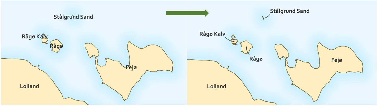
There are several new renderers in QGIS and some enhancements to existing renderers. One just introduced at v3.20 Odense is the Merged Features renderer. This renderer can be used with both polygon and line layers. It essentially renders the features as if they were dissolved into a single feature. Below I show it being applied to Danish Municipality polygons. The result is a single polygon for Danmark. This can be helpful in situations where a dissolved feature is needed simply for cartographic purposes. In this way it is similar to the Heat Map renderer for points. By using it, you can avoid creating another layer just for visualization purposes.

Interpolated Lines

Another notable addition introduced in 3.20 Odense, is a Symbol layer type renderer called Interpolated Lines. It creates a line with continuously varying color and/or width. The symbol is highly configurable. It has data defined overrides exposed for all settings.

One “use case”, is tapering streams in stream network, based on Strahler Order. In the example below, the Varying width option is being used. Here the line width is determined using the attribute columns containing Strahler Order data (Start & End values). There are also options to set the Minimum and Maximum line width.

This is just one example. You can set the Width to be Fixed or Varied as well as the Color. When using a Varying color you can use the color ramp widget.

Label Callouts

Labeling has had numerous improvements in the last year, especially with the release of QGIS 3.20 Odense. First introduced in QGIS 3.10, label callouts are a great option when the label text will not fit within the polygon. See the example below.

Now in 3.20 you will see two new options for configuring label callouts: Curved lines and Balloons (speech bubbles).

If you choose the Curved lines option you can specify:

• the amount of Curvature applied to the callout lines - increasing the value increases the curvature
• the Orientation (automatic, clockwise or counterclockwise) of the curvature

Using the Labels toolbar It is also possible to manually edit the location of both the label text and the beginning and ending of each callout line. This makes it very easy to place them just the way you want them. The location values are automatically stored in the project database via Data defined overrides.

If you choose the Balloon callouts option you can control:

• the Margins around the label text to the Balloon edge
• the Corner radius - increasing the value creates more rounded corners
• the Wedge width of the callout leader line - increasing the value increases the thickness on the balloon side of the leader line.

Note: Blending modes have also been exposed for all label callout types.

Print Layouts

There have been numerous changes to print layouts in the last year. This spring I wrote a blog post on custom QGIS Legend Patches. Another interesting new feature related to Print layouts is Clip Maps to Shape. QGIS 3.16 Hannover introduced a Clipping setting in the Item Properties for your map in a print composition. This allows you to clip your map to a shape and create a non-rectangular map.

• In the Print composer, add the shape you wish to use for clipping the map.
• Select the map object, and find the Clip Settings button on the Item Properties panel.
• Select Clip to Item and select the clipping object.

In the example below, an ellipse is added and used as the Clipping shape. This can really make a map stand out from an array of ordinary rectangular maps!

Note: This feature can also be used when working with an Atlas to clip the map to the current atlas feature!

Point Cloud Support

The last feature I will cover is point cloud support. This is certainly one of the most exciting advances in the last year. At version 3.18 Zurich, QGIS introduced support for both file based (LAS/LAZ) and cloud based (EPT) point clouds. Here I will focus on how these data can be visualized. Point clouds can be rendered four ways:

• The default is Extent only which shows the footprint of the dataset as a dashed red line.
• Point cloud datasets can also be visualized as an Attribute by Ramp. This is great for showing elevations (Z values) in the data with a color ramp.
• There is an RGB renderer. In the example below RGB values have been obtained by using the plugin LAS Tools to get RGB values from an aerial photo.
• Lastly, you can show the Classification of the point cloud data if that field exists in the data.

Point Clouds in 3D

It is also possible to view Point Cloud data in the QGIS 3D viewer. QGIS automatically identifies the heights. In the example below, two additional new QGIS features are demonstrated: rendering Shadows and Eye Dome Lighting. Both options can help to distinguish features in the scene.

Note: It is also now possible to Export a 3D scene for further visualization in softwares such as Blender.

Want to learn more about the best new features in QGIS?

You can learn more about new features added in the last year by watching my talk at the upcoming FOSS4G 2021 online conference. It is called: The Very Best New Features of QGIS 3.x. In this talk I will cover all types of new features introduced in the last year, with examples of each. It is scheduled for 30. September at 13:00 CET.

Want to learn more about data visualization and cartography with QGIS?

If you are interested in learning more about data visualization and cartography in QGIS, then sign up for the Data Visualization course, which starts on 1. December.

We also have a large number of other QGIS courses, you can read more about them here.